Debugging Shared Libraries with Binary Ninja
Sept 23 2018
Performing dynamic analysis on embedded system firmware can greatly improve the speed of the reverse engineering process. Disassemblers are essential for static analysis, but can also be used during dynamic analysis. While debugging during dynamic analysis is usually pretty straight forward in most disassemblers, they don't seem to offer an obvious way to follow the program flow when the application you are working on jumps to a shared library. Being able to follow that shared library jump in the disassembler allows you to better understand the program flow, and could help with patching the shared library if needed. There are a few issues that need to be solved before this is possible. First the memory location of the shared library will be unknown until the application or process has been started, and second the disassembler will treat the application and shared library as separate instances. So in order to use the disassembler for debugging while running dynamic analysis we will need a way to work around these issues. Below, I will introduce a simple technique for performing dynamic analysis of shared libraries using gdb, Binary Ninja, Voltron, and binjatron a plugin for Binary Ninja that allows for visual debugging during dynamic analysis.
Setup
Since most of my work involves embedded system RE, this example will focus on an approach that would be used for remote debugging of an embedded system target. I will include the setup process on the target side for repeatability purposes. However, this process will be dependant upon the interfaces you have available on your target. In this case, my target will be a Raspberry Pi running Linux raspberrypi 4.14.50+. I have installed gdbserver though the raspbian repo and I will use a tcp connection to connect to the gdbserver. I also have Binary Ninja, Voltron, and binjatron installed on my analysis computer. The installation process for Voltron or binjatron can be viewed on their github pages.
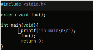
The example program is straight forward. A simple shared library compiled with '-fpic -c' and '-shared'. A main program which calls a function in the shared library which is then compiled with the location and name of the library. Below shows the results and source.

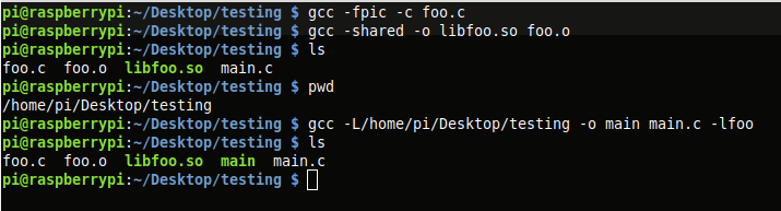
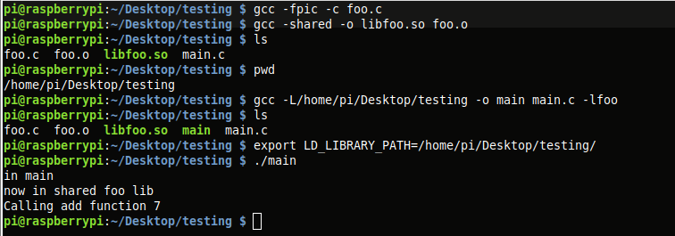
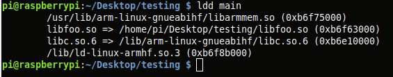
After compiling, LD_LIBRARY_PATH is set and the program is run. I also run 'ldd' to verify that the program is expecting libfoo as a shared lib.
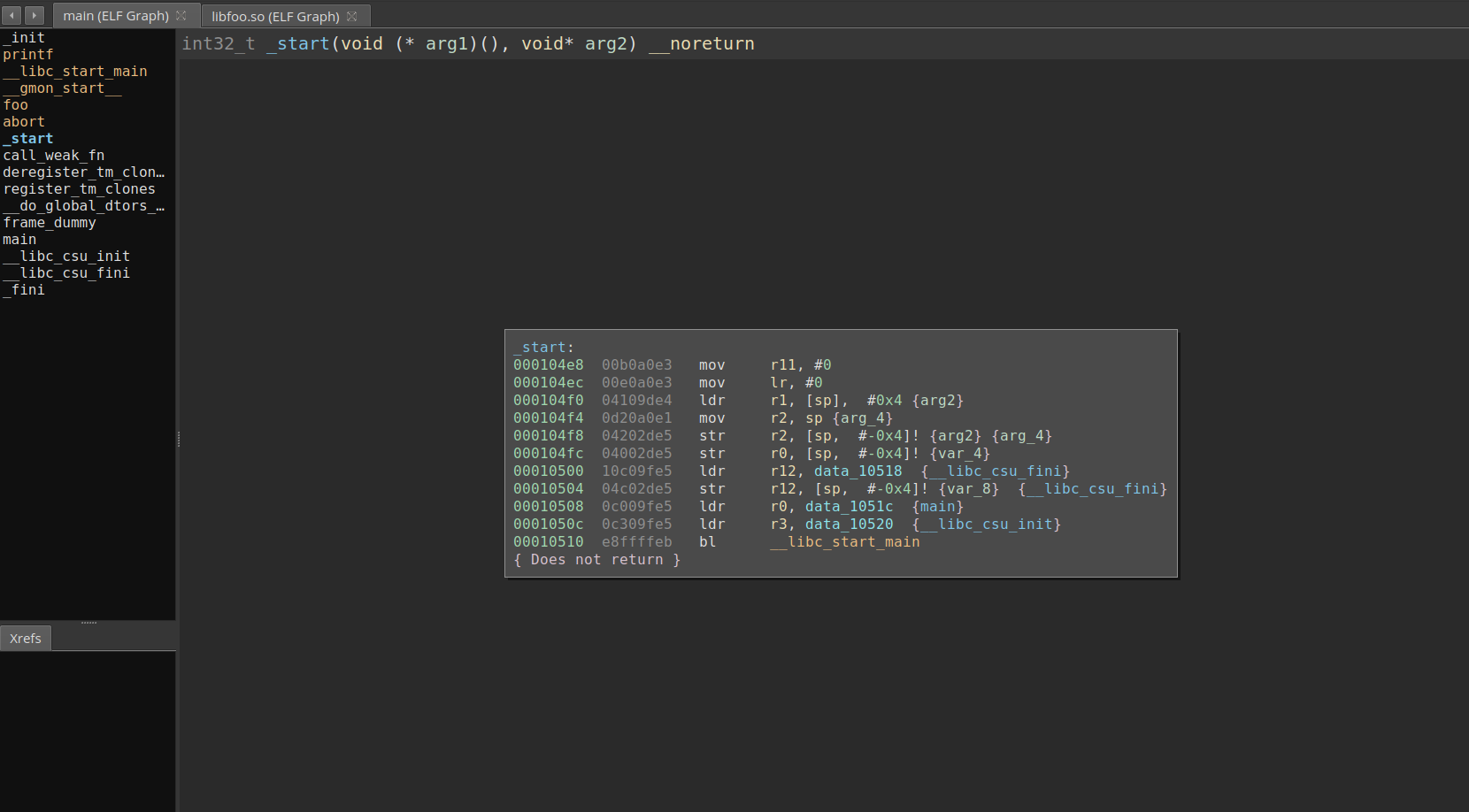
Pulling these programs into Binary Ninja we can verify things look correct. Below we can see the main program, and the foo shared library loaded into binary ninja using medium IL view on the libfoo.so.

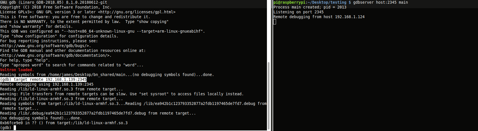
Everything looks correct so now I can start the gdbserver on the target using 'gdbserver host:2345 main. To connect to session you will need a gdb capable of performing cross architecture debugging. I have used 'arm-linux-gnueabihf-gdb' in the past and it seems to work here. Inside of gdb use 'target remote target-ip:2345' to make the connection.
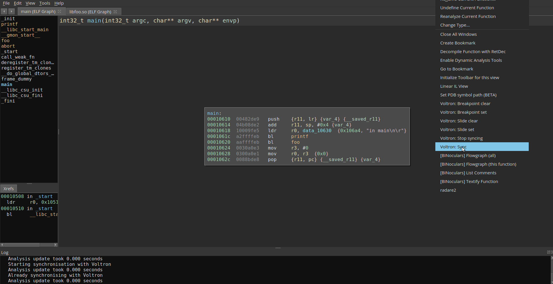
After the connection has been made, we can go back to Binary Ninja and sync to the Voltron session.
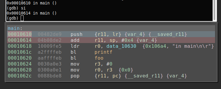
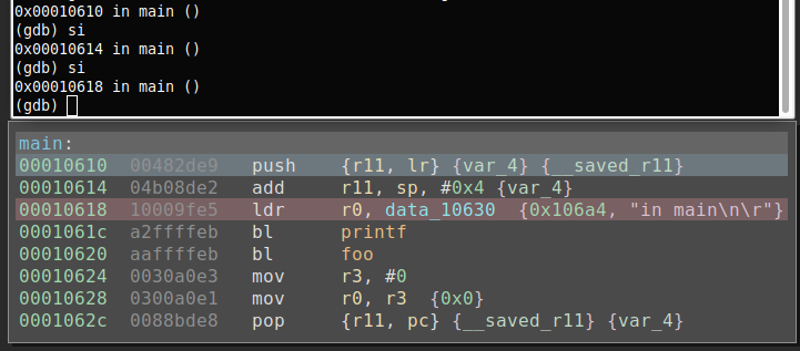
In order to verify the sync is working correctly, I set a breakpoint in main and step though.
Stepping though the program in gdb, binjatron will highlight the current PC in Binary Ninja which can be seen below.
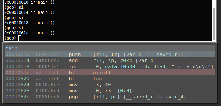
If we continue this until we get to foo() in plt setting up to make the external function call. More information on this can be found in this article.
Finding the shared library memory location
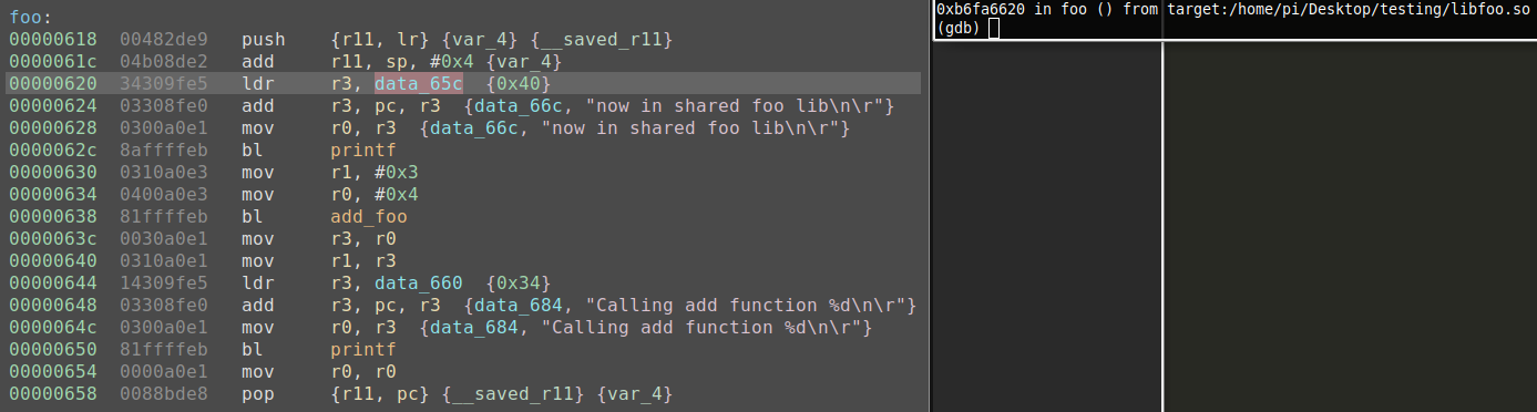
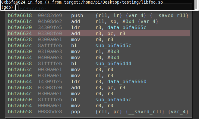
Now that I have verified everything is working nicely together, I can begin the setup process and perform dynamic analysis on the shared library. As stated earlier, if I simply continued stepping the application, once main calls foo() I will lose the current instruction highlighting due to the shared library code not being in the application's binary. Gdb and voltron alone could be used to perform dynamic analysis, but in larger functions with switch tables, having a graph view can give you a better understanding of the flow. You could also use the gdb/voltron output to manually follow along with the disassembly in Binary Ninja, but making it all work together in one view can have it's advantages by speeding up the process. The biggest issue here is getting the shared library offset synced in Binary Ninja with where the application expects the code. The voltron link will not sync since the address is offset. The simple solution is to offset the loading address of the shared library and resync voltron and that is what we are going to do. First the file offset needs to be obtained somehow. While there can be many ways to do this, in this case I simply place a breakpoint at foo(). Your approach could be different. Below we can see this breakpoint gives us an address of 0xb6fa6620.
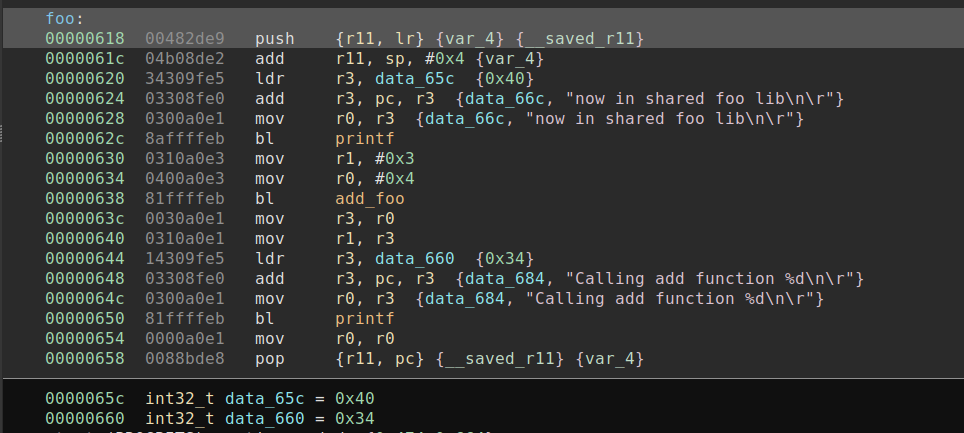
Analyzing the library in Binary Ninja we see the 0x620 offset is in foo() after the stack has been saved going into the function call. We can now use this information to calculate where we should offset the starting address, 0xb6fa6620 - 0x620 = 0xb6fa6000.
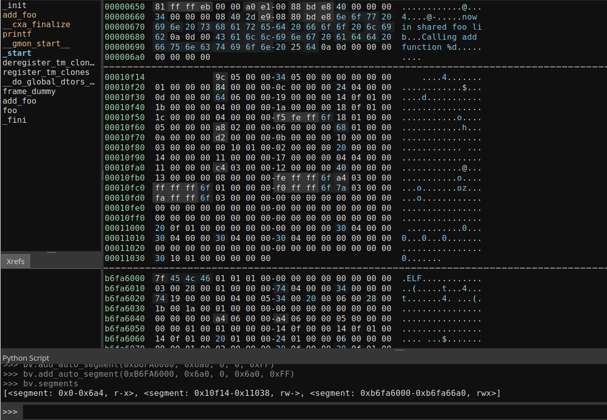
While Binary Ninja has no obvious way to rebase the binary using the user interface, it does have an api call that seems to do the trick. While they don't give an example or description of the call, add_auto_segment seems to copy data from the current selected file, and give it an offset. In this instance, for add_auto_segment(self, start, length, data_offset, data_length, flags): start will be our offset address of 0xb6fa6000, length will be the original file length, data_offset will be 0, and data_length will be the original file length. I also pass in 0xff for flags to make the segment writable, readable, and executable. The final command will be 'bv.add_auto_segment(0xb6fa6000, 0x6a0, 0, 0x6a0, 0xFF)'. Below you can see the results of running the command in Binary Ninja's python console.
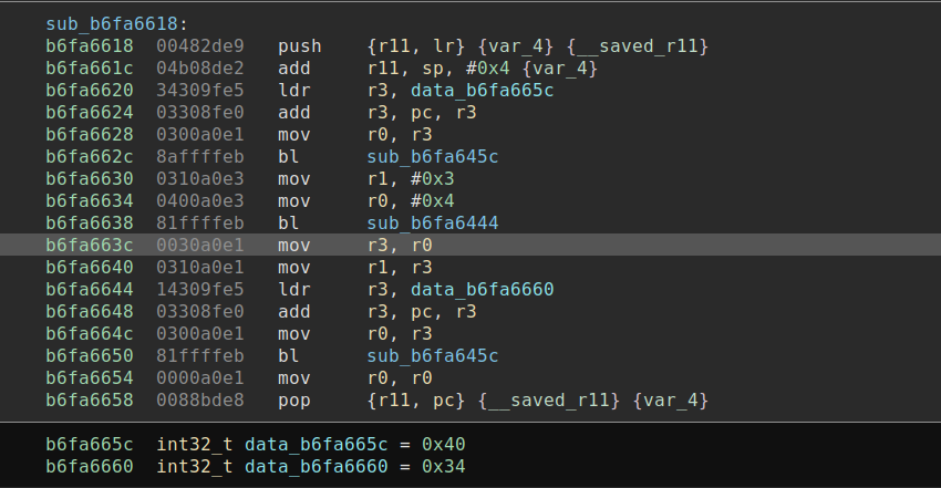
Creating functions in the new segment is the last step before we can continue with the dynamic analysis. Doing this is as easy as scrolling to the offset of the function in Binary Ninja's linear view in the new segment and pressing 'p'. Binary Ninja will analyze the newly created function, and do recursive analysis of the calls in the new segment. I have not yet been able to get the linear sweep analysis mode to work, however this could be an alternative. Below, you can see the original foo() compared to the offset foo().
Wrapping up and what happens next
I have the offset calculated, functions created at the offset, and now I am ready to continue with dynamic analysis. First I need to stop syncing and resync with the shared library disassembled instance in Binary Ninja. This is again done by right clicking in Binary Ninja and choosing 'Voltron: Stop Syncing' / 'Voltron: Sync'. Once I do that I can start stepping though using gdb and see the current instruction highlighted as before.


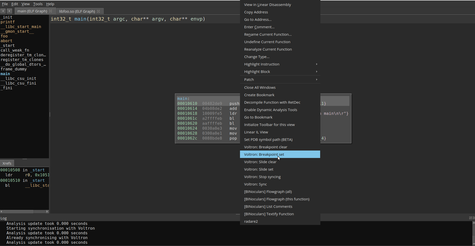
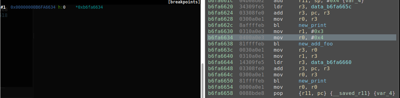
I can also use the Binary Ninja binjatron to set breakpoints in the shared library now as well.
While calculating the offset and using Binary Ninja's python console is simple and straight forward. Having a plugin that could automatically perform these actions for the person performing analysis would greatly speed up this process. This would especially be needed for applications that relied on multiple shared library calls in which dynamic analysis are desired.